Visualization
This page provides examples of how to visualize membrane curvature via Matplotlib. Two different approaches are suggested.
Warning
Please note that when plotting via imshow() or
contourf(), the orientation of the plot in the
final rendering is determined by the origin argument. By default,
in these Matplotlib functions, the origin is set to the (left, top)
corner. Additionally, for an array of shape (M, N), the first index
M runs along the vertical axis, and the second index N runs along
the horizontal axis.
For these reasons, the returned arrays of surface, mean, and Gaussian
curvature should be transposed, and origin=lower should be passed to
imshow() or contourf()
to generate the correct plots. This is a critical step when visualizing
results obtained from MembraneCurvature analyses to avoid generating
plots of membrane surface and curvature with the wrong orientation.
1. imshow
A simple plot using imshow() can be obtained like so:
import matplotlib.pyplot as plt

fig, ax = plt.subplots()
ax.imshow(avg_mean_curvature.T, cmap='bwr', interpolation='gaussian', origin='lower')
ax.set_title('Mean Curvature')
plt.show()
With imshow(), each element of the array is plotted as
a square in a matrix of M x N elements. Since we are interested in plotting
the array wwhere the first index runs along the horizontal axis, while the
second index runs along the vertical, we should transpose the array obtained
from the MembraneCurvature analysis. In the generated plot, the color of each
square is determined by the value of the corresponding array element and the
colormap of preference.
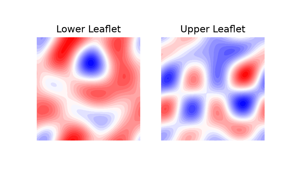
For example, to visualize the results obtained in 2.1. Membrane-only systems, we can run:
In [1]: import MDAnalysis as mda
   ...: from membrane_curvature.base import MembraneCurvature
   ...: from MDAnalysis.tests.datafiles import Martini_membrane_gro
   ...: import matplotlib.pyplot as plt
   ...:

In [2]: universe = mda.Universe(Martini_membrane_gro)

In [3]: curvature_upper_leaflet = MembraneCurvature(universe,
   ...:                                             select='resid 1-225 and name PO4',
   ...:                                             surface_method='binning',
   ...:                                             n_x_bins=8,
   ...:                                             n_y_bins=8,
   ...:                                             wrap=True).run()
   ...:

In [4]: mean_upper_leaflet = curvature_upper_leaflet.results.average_mean

In [5]: curvature_lower_leaflet = MembraneCurvature(universe,
   ...:                                             select='resid 226-450 and name PO4',
   ...:                                             surface_method='binning',
   ...:                                             n_x_bins=8,
   ...:                                             n_y_bins=8,
   ...:                                             wrap=True).run()
   ...:

In [6]: mean_lower_leaflet = curvature_lower_leaflet.results.average_mean

In [7]: leaflets = ['Lower', 'Upper']

In [8]: curvatures = [mean_lower_leaflet, mean_upper_leaflet]

In [9]: fig, [ax1, ax2] = plt.subplots(ncols=2, figsize=(6,3), dpi=200)
   ...: for ax, mc, lf in zip((ax1, ax2), curvatures, leaflets):
   ...:     ax.imshow(mc.T, origin='lower', interpolation='gaussian', cmap='seismic')
   ...:     ax.set_aspect('equal')
   ...:     ax.set_title('{} Leaflet'.format(lf))
   ...:     ax.axis('off')
   ...:
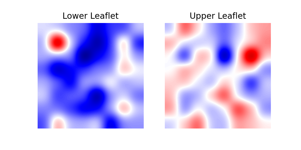
Alternatively, with the Fourier method and the default values for the fit, we can run:
In [10]: import MDAnalysis as mda
   ....: from membrane_curvature.base import MembraneCurvature
   ....: from MDAnalysis.tests.datafiles import Martini_membrane_gro
   ....: import matplotlib.pyplot as plt
   ....:

In [11]: universe = mda.Universe(Martini_membrane_gro)

In [12]: curvature_upper_leaflet_fourier = MembraneCurvature(universe,
   ....:                                                     select='resid 1-225 and name PO4',
   ....:                                                     surface_method='fourier',
   ....:                                                     ).run()
   ....:

In [13]: mean_upper_leaflet_fourier = curvature_upper_leaflet_fourier.results.average_mean

In [14]: curvature_lower_leaflet_fourier = MembraneCurvature(universe,
   ....:                                                     select='resid 226-450 and name PO4',
   ....:                                                     surface_method='fourier',
   ....:                                                     ).run()
   ....:

In [15]: mean_lower_leaflet_fourier = curvature_lower_leaflet_fourier.results.average_mean

In [16]: leaflets = ['Lower', 'Upper']

In [17]: curvatures_fourier = [mean_lower_leaflet_fourier, mean_upper_leaflet_fourier]

In [18]: fig, [ax1, ax2] = plt.subplots(ncols=2, figsize=(6,3), dpi=200)
   ....: for ax, mc, lf in zip((ax1, ax2), curvatures_fourier, leaflets):
   ....:     ax.imshow(mc.T, origin='lower', interpolation='gaussian', cmap='seismic')
   ....:     ax.set_aspect('equal')
   ....:     ax.set_title('{} Leaflet'.format(lf))
   ....:     ax.axis('off')
   ....:
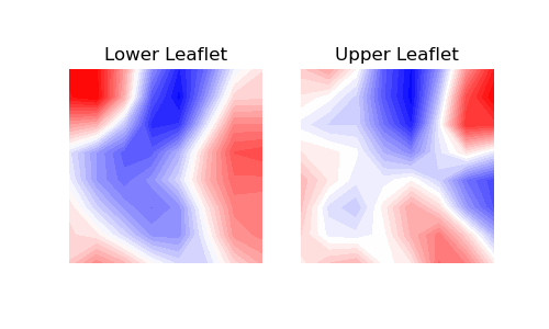
2. contourf
You can use contour plots using contourf(). With this
approach, contour lines and filled contours of the obtained two-dimensional data
are plotted. A contour line connects points with the same curvature values.
When plotting using contourf(), an extra step is required
to perform an interpolation. We suggest using
scipy.ndimage.gaussian_filter() as in:
In [19]: from scipy import ndimage

In [20]: leaflets = ['Lower', 'Upper']

In [21]: fig, (ax1, ax2) = plt.subplots(ncols=2, figsize=(5,3), dpi=200)
   ....: for ax, mc, lf in zip((ax1, ax2), curvatures, leaflets):
   ....:     arr_ = ndimage.gaussian_filter(mc, sigma=1, order=0, mode='reflect')
   ....:     ax.contourf(arr_.T,
   ....:                 cmap='bwr',
   ....:                 levels=30)
   ....:     ax.set_aspect('equal')
   ....:     ax.set_title('{} Leaflet'.format(lf))
   ....:     ax.axis('off')
   ....:
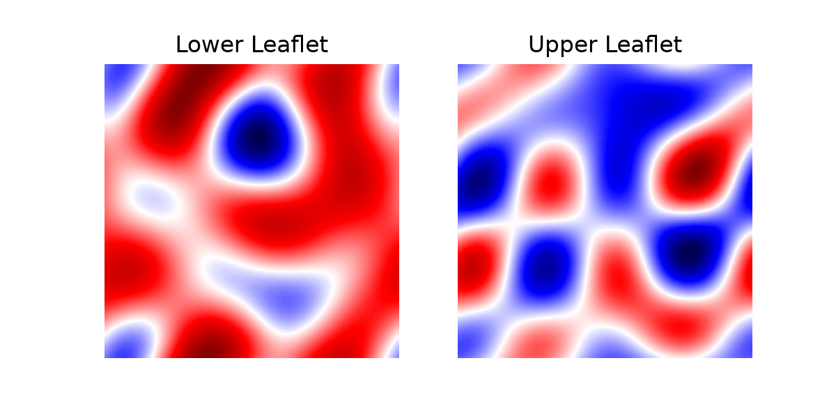
Or with the Fourier method:
In [22]: from scipy import ndimage

In [23]: leaflets = ['Lower', 'Upper']

In [24]: fig, (ax1, ax2) = plt.subplots(ncols=2, figsize=(5,3), dpi=200)
   ....: for ax, mc, lf in zip((ax1, ax2), curvatures_fourier, leaflets):
   ....:     arr_ = ndimage.gaussian_filter(mc, sigma=1, order=0, mode='reflect')
   ....:     ax.contourf(arr_.T,
   ....:                 cmap='bwr',
   ....:                 levels=30)
   ....:     ax.set_aspect('equal')
   ....:     ax.set_title('{} Leaflet'.format(lf))
   ....:     ax.axis('off')
   ....: