Algorithm

Overview

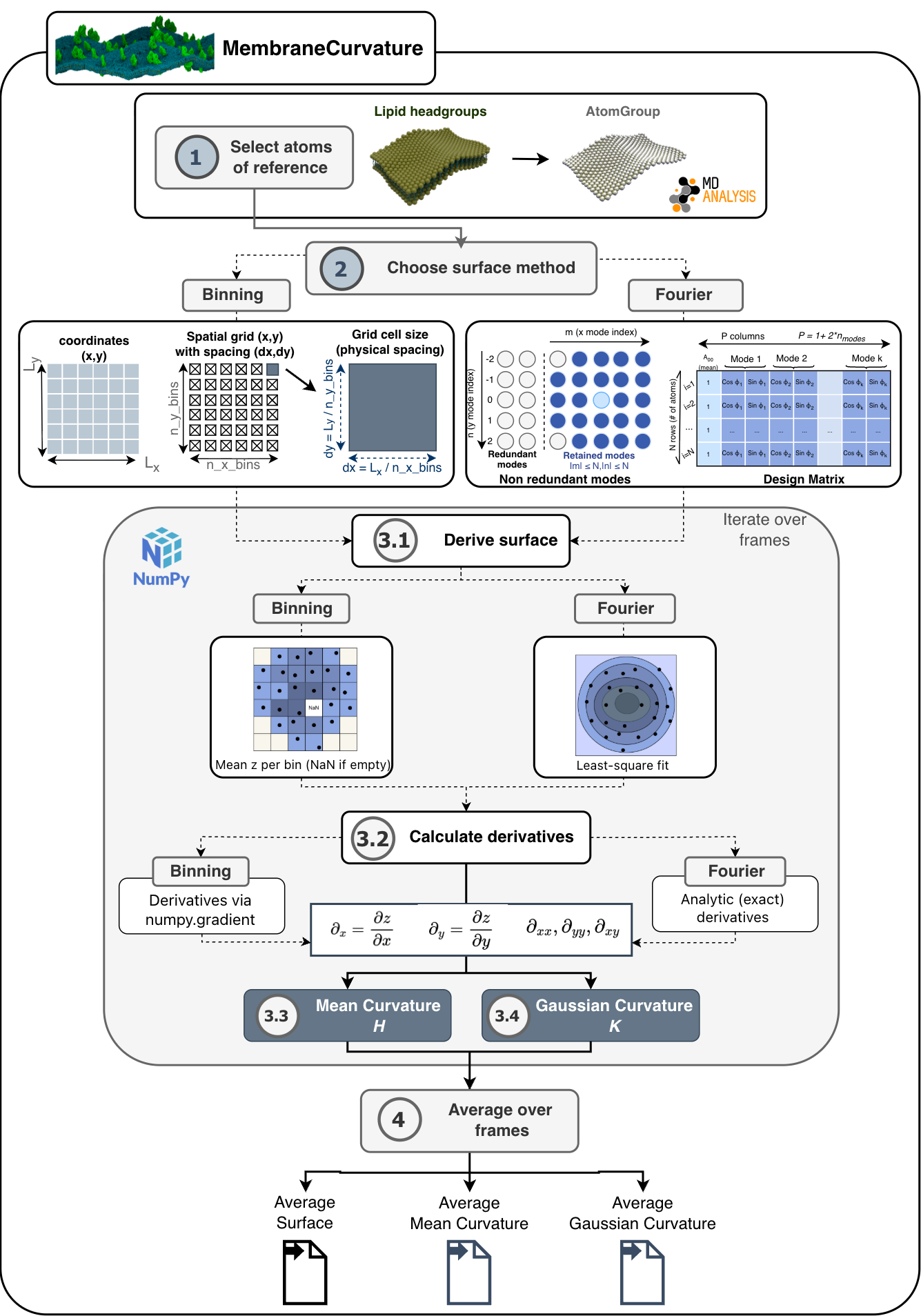
MembraneCurvature calculates mean and Gaussian curvature of surfaces derived from atoms of reference in 4 steps:

1. Select atoms of reference

2. Choose surface method

3. Derive surface and calculate surface derivatives

4. Average over frames

A summary of the algorithm used in MembraneCurvature is shown in the following diagram:

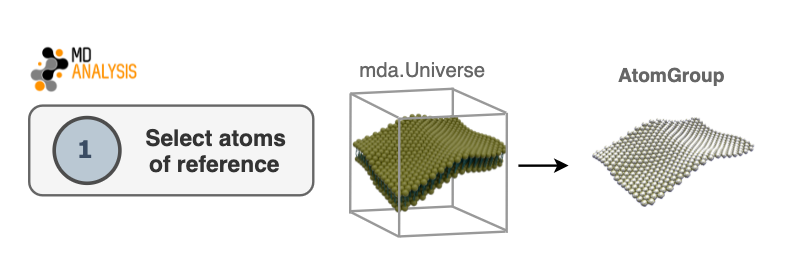
1. Select atoms of reference

The first step in the algorithm consists of selecting atoms that will be used as a reference to derive a surface. This selection will be contained in an AtomGroup. Typically in biological membranes, lipid headgroups are the most common elements to use as an AtomGroup of reference.

2. Choose surface method

Two surface-derivation methods are available, selected via the surface_method argument of MembraneCurvature.

• 2.1 Fourier method (surface_method='fourier', default method)

  A truncated 2D Fourier series is fitted to atom heights by linear least squares at each frame. Partial derivatives are evaluated analytically from the fitted series on the same grid as the binning method, avoiding finite-difference discretization error. See fourier_surface for details.

• 2.2. Binning method (surface_method='binning')

  Atoms are assigned to bins on a regular grid and the height of each bin is set to the mean \(z\)-coordinate of its atoms. Partial derivatives are estimated numerically from the discrete height field using numpy.gradient() with the physical bin spacing. See binning_surface for details.

2.1 Fourier method

surface_method='fourier' is the default method used in Membrane Curvature. The Fourier method fits a truncated periodic 2D Fourier series to atom heights by linear least squares at each frame. The truncation is controlled by fourier_m and fourier_n (default 2). The basis is periodic on the simulation box with periods \(L_x\) and \(L_y\), so the fitted surface is consistent with periodic boundary conditions in \(x\) and \(y\).

The Fourier expansion used as a basis function is given by:

\[z(x, y) = A_{00} + \sum_{m=1}^{M}\sum_{n=1}^{N}\left[ A_{mn}\cos\!\big(k_x m x + k_y n y\big) +\,B_{mn}\sin\!\big(k_x m x + k_y n y\big) \right].\]

Here, \(k_x\) and \(k_y\) are the fundamental wavevector components:

\[k_x = \frac{2\pi}{L_x}, \qquad k_y = \frac{2\pi}{L_y}\]

therefore the phase for the mode (m,n) is

\[(k_x m x + k_y n y).\]

The Fourier method in MembraneCurvature is conceptually related to Fourier surface modeling [CAG2009] and molecular Fourier shape descriptors [JMG1988], but it is not a direct implementation of either paper. The least-squares height-field fit used in MembraneCurvature is tailored to the AtomGroup of reference given their cordinates.

[CAG2009]

Shen et al., Fourier method for large-scale surface modeling and registration, Computers & Graphics (2009), doi: 10.1016/j.cag.2009.03.002.

[JMG1988]

Leicester et al., Description of molecular surface shape using Fourier descriptors, Journal of Molecular Graphics (1988), doi: 10.1016/0263-7855(88)85008-2.

The full Fourier surface workflow comprises six steps, where the first four steps build and solve a linear model that reconstructs the height field from plane-wave basis functions. The final two steps evaluate the fitted surface and its derivatives analytically on a grid of bin centres. In the following sections, we describe the overall workflow implemented in MembraneCurvature. For details on each step and the associated functions, see the API documentation in fourier_surface.

2.1.1 Choose Fourier modes

The first step is to choose a non-redundant set of Fourier modes with fourier_mode_list() and determine the total parameter count with n_fourier_parameters(). This removes conjugate redundancy for real-valued surfaces and isolates the mean term.

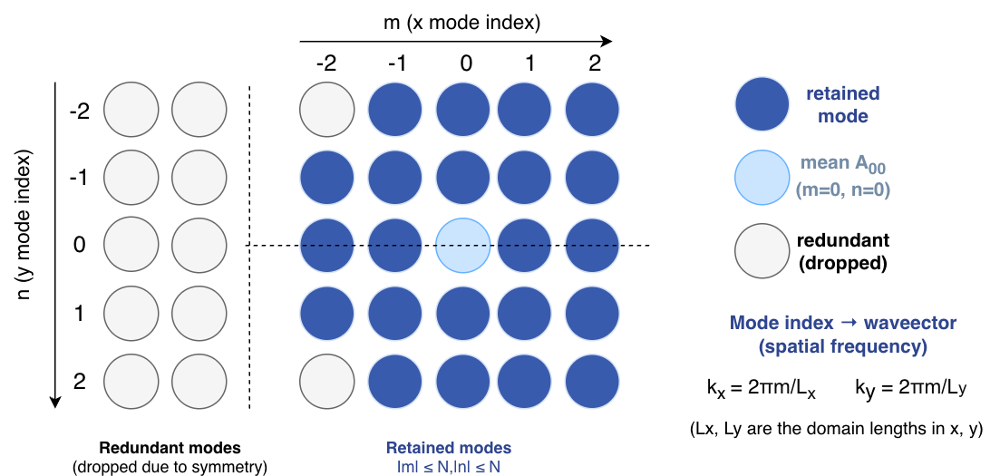
2.1.2 Compute wavevectors

We then compute the wavevector components (\(k_x\), \(k_y\)) for each mode using _compute_wavevector(). These set the phase \(\phi = k_x x + k_y y\) that appears in each cosine/sine basis function.

MembraneCurvature builds the non-redundant mode list via fourier_mode_list(M, N)() and computes the total parameter count with n_fourier_parameters(M, N)(). MembraneCurvature then validates that the AtomGroup of reference contains at least that many atoms and raises a ValueError if the selection is too small.

Warning

The explanation above is for the users to understand how MembraneCurvature builds the mode list and parameter count internally.

Do not pass the mode list fourier_mode_list(M, N)() or parameter count n_fourier_parameters(M, N)() directly. MembraneCurvature builds them internally.

Users choose the Fourier truncation via the constructor arguments fourier_m and fourier_n By passing the maximum mode indices, MembraneCurvature builds the actual mode list and computes the total parameter count.

Important

Because the derivatives are analytic, the Fourier method is not subject to finite-difference discretization error from the bin grid. Curvature still depends on the Fourier series truncation: use fourier_m = fourier_n = 2 unless shorter wavelengths are required, and increase these values only while curvature improves systematically rather than becoming dominated by noise.

2.1.3 Build design matrix

We then build the design matrix with _build_fourier_matrix(). Each row of the design matrix corresponds to an atom position and columns are the constant offset followed by \(\cos(\mathbf{k}\cdot\mathbf{r})\), \(\sin(\mathbf{k}\cdot\mathbf{r})\) pairs for every retained mode. This matrix encodes the linear relation between the Fourier coefficients and the observed heights.

The design matrix \(\mathbf{\Phi}\) is a matrix of shape \((N, P)\) where \(N\) is the number of atoms in the AtomGroup of reference, and \(P\) is the number of parameters. \(P\) is defined as \(P = 1 + 2\,n_{\text{modes}}\) where \(n_{\text{modes}}\) is the number of the k retained Fourier modes.

We can conceptualize \(\mathbf{\Phi}\) as a matrix with rows corresponding to atom positions and columns corresponding to the basis functions (cosine and sine of the wavevector \(k\)) evaluated at each atom position, so that the fitted heights satisfy the linear system of equations \(\mathbf{z} \approx \mathbf{\Phi}\,\boldsymbol{\theta}\), from which we can solve for the Fourier coefficients by solving a least-squares system.

A single row \(i\) of \(\mathbf{\Phi}\) for an atom at \(\mathbf{r}_i=(x_i,y_i)\) has the form:

\[\begin{split}\begin{aligned} \mathbf{\Phi}_{i,:} = \big[\, & 1, \\ & \cos\big(\phi_{m_1,n_1}(\mathbf{r}_i)\big),\; \sin\big(\phi_{m_1,n_1}(\mathbf{r}_i)\big), \\ & \ldots, \\ & \cos\big(\phi_{m_{k},n_{k}}(\mathbf{r}_i)\big),\; \sin\big(\phi_{m_{k},n_{k}}(\mathbf{r}_i)\big) \,\big] \end{aligned}\end{split}\]

With this formulation, we can solve for the Fourier coefficients by solving a least-squares system:

\[\mathbf{z} \approx \mathbf{\Phi}\,\boldsymbol{\theta}\]

where \(\boldsymbol{\theta}\) is the vector of Fourier coefficients. These coefficients are the ones we use to reconstruct the height field and calculate the derivatives.

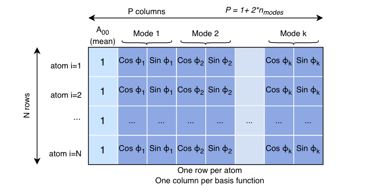
Note that the column ordering follows the mode list returned by fourier_mode_list(). For each retained mode (m,n) the design matrix contains a cosine column then a sine column, so columns appear as 1, cos_{(m1,n1)}, sin_{(m1,n1)}, cos_{(m2,n2)}, sin_{(m2,n2)}, ....

Important

In summary:

The design matrix \(\mathbf{\Phi}\) has shape \((N, P)\) where rows (\(N\)) are atoms and columns (\(P\)) are the basis functions. \(N\) is the number of atoms in the AtomGroup of reference. \(P\) is the total number of parameters:

\[P = 1 + 2\,n_{\text{modes}}\]

which is the sum of one constant column (the mean term \(A_{00}\)) plus two columns for each retained Fourier mode (one for cosine and one for sine).

2.1.4 Solve least-squares system

We then solve the least-squares system for the Fourier coefficients using _fourier_fit_from_atoms(), which calls _solve_design_least_squares_svd(). The latter function solves the linear least-squares system via truncated SVD.

This function solves the least-squares system for the Fourier coefficients and splits the solution vector into the mean term \(A_{00}\) and the per-mode amplitudes \(A_{mn}\) and \(B_{mn}\) with _unpack_coefficients(). The returned coefficients are then used to evaluate the fitted height and its analytic derivatives on the bin-centre mesh via _eval_fourier_surface().

The Fourier coefficients are obtained by linear least squares. The coefficients are obtained by minimizing the residual sum of squares between the observed heights and the fitted heights:

\[\hat{\boldsymbol{\theta}} = \operatorname{arg\,min}_{\boldsymbol{\theta}} \lVert \mathbf{\Phi}\,\boldsymbol{\theta} - \mathbf{z} \rVert_2^2\]

via truncated SVD (_solve_design_least_squares_svd()). Because the model is linear in \(\boldsymbol{\theta}\), no nonlinear optimisation is required. If the effective rank of \(\mathbf{\Phi}\) is smaller than \(P\), a UserWarning is emitted. The truncated-SVD solver still returns a well-defined minimum-norm least-squares solution, but the coefficients are not uniquely determined by the data.

Overall, truncated SVD lets us fit the best surface even when the data can’t uniquely determine every Fourier coefficient, and it reduces noise amplification in modes that are not well-determined by the data.

2.2. Binning method

The binning method derives a surface by partitioning the simulation box into a regular n_x_bins x n_y_bins grid along the \(x\) and \(y\) directions. For each bin we compute the average \(z\) coordinate of the atoms that fall inside the bin to form the discrete height field.

The resulting discrete height field is then differentiated numerically using numpy.gradient() to obtain the partial derivatives required for curvature calculation. Set surface_method='binning' explicitly to use this method; it requires no additional parameters beyond the grid dimensions.

In the next section, we describe the details of the binning method.

2.2.1. Set grid

The dimensions of the grid are determined by the size of the simulation box contained in the Universe. The grid covers a rectangular domain in the membrane plane. By default that domain matches the x and y edges of the simulation box from MDAnalysis’ Universe. The grid comprises n_x_bins x n_y_bins bins along the x and y directions. Note that the user can define the number of bins via the n_x_bins and n_y_bins arguments.

For every atom in the AtomGroup of reference, MembraneCurvature assigns it to a grid cell based on its x and y coordinates. In practice, each coordinate pair (x, y) is mapped to a grid location [l, m] corresponding to a bin in the discretized membrane surface.

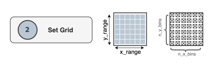
Here, \(L_x\) and \(L_y\) denote the size of the simulation box in the x and y directions, respectively, while the size of the region covered by the grid is represented by x_range and y_range, along the x and y directions, respectively. The spacing between grid points in each direction is then determined by dividing these lengths by the number of bins.

Note

Unless the user provides a different input, MembraneCurvature will determine the dimensions of the grid based on the size of the box on the first frame via dimensions.

grid_dimension_x = (0, universe.dimensions[0])
grid_dimension_y = (0, universe.dimensions[1])

2.2.2. Populate grid

Once the grid has been populated, the z coordinates of atoms assigned to each cell are collected to form a height field over the grid.

Coordinates are converted to integer bin indices via scale factors

\[x\_factor = \frac{n\_{x\_bins}}{x_{\max} - x_{\min}}, \qquad y\_factor = \frac{n\_{y\_bins}}{y_{\max} - y_{\min}}.\]

We histogram the atoms of reference into a 2D grid by mapping each atom at \(x\) and \(y\) coordinates to an integer bin index. The scale factor converts coordinates from length units into bin units so that flooring yields an integer index:

\[\mathrm{index} = \left\lfloor (x - x_{\min})\,x\_factor \right\rfloor,\]

and similarly for \(y\).

Atoms that map outside the valid bin range (negative indices or indices ≥ n_x_bins/n_y_bins) are skipped and trigger a one-time detailed warning. The function uses a WarnOnce helper so the full diagnostic is shown on first occurrence and a short message on subsequent occurrences.

To populate the grid, MembraneCurvature wraps the coordinates of the AtomGroup of reference using wrap() only when wrap=True is set (the default for surface_method='binning').

Empty bins (zero samples) are represented as numpy.nan in the returned (n_x_bins, n_y_bins) array: the implementation replaces zero counts with numpy.nan and divides summed z-values by the per-bin counts. As a result, trajectory averages use numpy.nanmean() and therefore ignore empty bins.

Warning

The binning routine itself does not apply periodic wrapping; MembraneCurvature applies AtomGroup.wrap() only when wrap=True is set.

• Set wrap=True to pack atoms back into the grid if you are calculating curvature on a raw trajectory.

• Set wrap=False to omit atoms from the simulation box that fall outside the grid when you are calculating curvature on:

  • a trajectory (membrane only or membrane-protein with position restraints) that already pre-processed periodic boundary conditions.

  • a membrane-protein system that already pre-processes rotational and translational fit for the protein.

3. Derive surface and calculate surface derivatives

For every frame of the trajectory, the surface derived from the AtomGroup is calculated and stored in z_surface. Similarly, the calculation of mean and Gaussian curvature is performed in every frame and stored in MembraneCurvature.results.mean and MembraneCurvature.results.gaussian, respectively.

The following sections describe the details of the two methods used to derive the surface and calculate its derivatives.

3.1. Derive surface

The surface is derived from atom positions using the selected method and stored in z_surface for each frame.

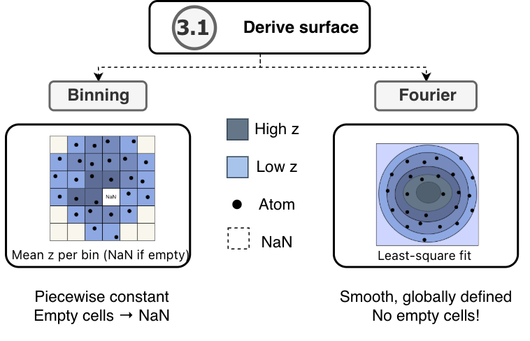
With surface_method='binning', the height field is the discrete \(N_x \times N_y\) array of per-cell mean \(z\) coordinates assembled in 2.2.1. Set grid. Bins containing no atoms are set to NaN and excluded from trajectory averages.

With surface_method='fourier', the height field is the fitted Fourier series evaluated at bin centres after the least-squares fit described in 2.1 Fourier method. Because the representation is continuous and periodic on the simulation box, every bin centre receives a value and no NaN entries arise.

3.2. Calculate derivatives

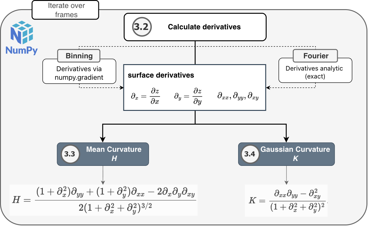
Five partial derivatives of the height field are required by the curvature formulas: the first derivatives \(\partial_x\) and \(\partial_y\), the second derivatives \(\partial_{xx}\) and \(\partial_{yy}\), and the mixed derivative \(\partial_{xy}\).

Important

There is a key difference between the binning and Fourier methods when it comes to calculating the derivatives!

• With the binning method, the derivatives are estimated numerically from the discrete height field using numpy.gradient() with the physical spacings \(\Delta x\) and \(\Delta y\), so that curvature values are in physical units.

• With the Fourier method, the derivatives are evaluated analytically from the fitted Fourier series, so they are not subject to finite-difference discretization error. Curvature accuracy is instead governed by the Fourier series truncation.

Therefore, the two methods differ in what limits curvature accuracy: binning is sensitive to finite-difference error on the height grid (often worse when the grid is coarse), while the Fourier pipeline is sensitive to how well the truncated series fits the atom data; its derivatives are exact for that fitted surface at any output grid resolution, so refining the bin grid alone does not remove truncation or sampling limitations.

3.2.1. Binning + finite differences (surface_method='binning')

With surface_method='binning', these are estimated numerically from the discrete height field using numpy.gradient() with the physical spacings \(\Delta x\) and \(\Delta y\), so that curvature values are in physical units. Because this step uses finite differences, very coarse grids may introduce discretization error.

Note

These derivatives are evaluated using the actual grid spacing (dx, dy), so that changes in height are measured per unit distance in real space rather than per grid index. This makes curvature values physically meaningful and reduces their sensitivity to the chosen grid resolution.

Curvature is computed from surface derivatives evaluated using the grid spacing (dx, dy), ensuring results are expressed in physical units and are less sensitive to grid resolution. Because the derivatives are computed numerically, very coarse grids may still affect curvature estimates due to finite-difference discretization error.

For details on the binning method, see API documentation in binning_surface that describes every associated functions.

3.2.1.1. FFT filtering on the averaged surface (fft_filter)

A brick-wall filter is applied to the averaged surface once all frames have been processed when surface_method='binning' and the argument fft_filter is set to 'auto' (default) or passed as a dictionary like {'q': (q_low, q_high)}.

Important

The FFT filter is not applied to per-frame surfaces. Filtering is performed on the time-averaged height field, where thermal fluctuations have already been suppressed by averaging.

Pass-band limits are resolved at construction time via resolve_fft_filter() and applied at the end of the run with apply_fft_filter() (see fft_filtering).

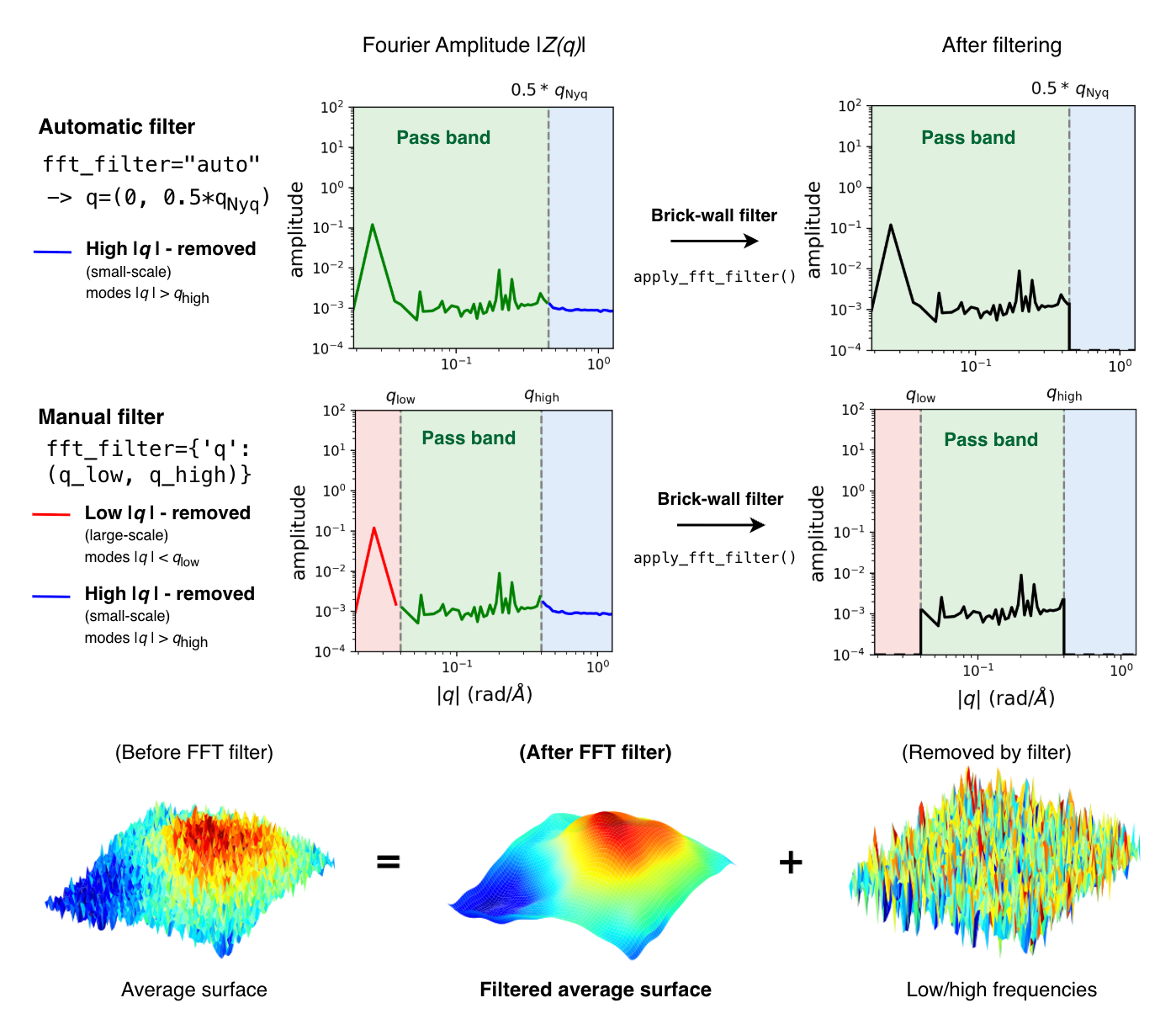
For filtered average surface maps, MembraneCurvature averages the height field (z_surface) over the trajectory and then smooths it in reciprocal space by zeroing all Fourier modes outside the pass band defined by \(q_{\mathrm{low}} \leq |q| \leq q_{\mathrm{high}}\) via apply_fft_filter() before transforming back to real space. The resulting filtered surface is stored in average_z_surface, and then used to calculate mean and Gaussian curvature via mean_curvature() and gaussian_curvature(), respectively.

With the default fft_filter='auto', the pass band is \((0,\ 0.5\,q_{\mathrm{Nyq}})\), a conservative low-pass by default which retains the large-scale membrane shape while suppressing short-wavelength noise.

For binning, filtering defaults to fft_filter='auto'. To control the band manually, pass fft_filter={'q': (q_low, q_high)} in rad/Å. To disable filtering altogether, pass fft_filter=None.

Warning

Before the FFT filtering, empty bins are temporarily filled with the mean height of occupied bins, then restored to NaN after the inverse FFT. Large empty regions can introduce broadband spectral contamination and distort the filtered surface near gaps. Prefer denser binning or smaller empty regions when filtering is enabled.

Note

The pass-band mask is isotropic in \(|q|\). For non-square bins (\(\Delta x \neq \Delta y\)), modes that are resolvable along the finer axis but exceed \(q_{\mathrm{Nyq}} = \min(\pi/\Delta x,\, \pi/\Delta y)\) are removed. Since numpy.fft.fft2() assumes a periodic grid, use wrap=True, as recommended for binning in general.

3.2.2. Fourier fit + analytic derivatives (surface_method='fourier')

With surface_method='fourier', the partial derivatives are evaluated analytically from the fitted Fourier series (see 2.1 Fourier method), so they are not subject to finite-difference discretization error. Curvature accuracy is instead governed by the Fourier series truncation.

Warning

Use fourier_m = fourier_n = 2 unless shorter wavelengths are needed, and increase the mode indices only while curvature improves systematically.

Note

Because no finite-difference step is involved, the analytic derivatives are exact with respect to the fitted surface, regardless of grid resolution.

For details on the Fourier method, see API documentation in fourier_surface that describes every step with its associated functions.

3.3. Mean curvature

Mean curvature \(H\) is calculated from the five partial derivative arrays using the Monge-gauge formula:

\[H = \frac{(1+\partial_x^2)\,\partial_{yy} + (1+\partial_y^2)\,\partial_{xx} - 2\,\partial_x \partial_y \partial_{xy}} {2\,(1+\partial_x^2+\partial_y^2)^{3/2}}\]

via mean_curvature_monge().

The result has units Å ^-1 and is stored in MembraneCurvature.results.mean for each frame.

3.4. Gaussian curvature

Gaussian curvature \(K\) is calculated from the same derivative arrays using:

\[K = \frac{\partial_{xx}\,\partial_{yy} - \partial_{xy}^2} {(1+\partial_x^2+\partial_y^2)^{2}}\]

via gaussian_curvature_monge().

As for the calculation of mean curvature, Gaussian curvature is calculated for every frame and the result has units Å ^-2 and is stored in MembraneCurvature.results.gaussian for each frame.

Warning

The Monge-gauge formulas in steps 3.3 and 3.4 are exact. There is no small-gradient approximation applied. Both methods feed the same five derivative arrays into the same formulas; the only difference is how those derivatives were obtained in step 3.2. Calculate derivatives.

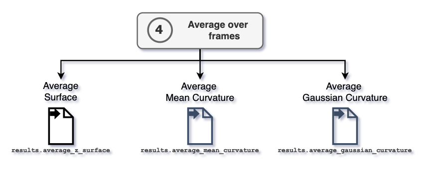
4. Average over frames

The attributes MembraneCurvature.results.average_mean and MembraneCurvature.results.average_gaussian contain the computed values of mean and Gaussian curvature averaged over all the n_frames in the trajectory.

After performing the average over frames, the information of average surface, mean, and Gaussian curvature are stored in the MembraneCurvature.results.average_z_surface, MembraneCurvature.results.average_mean, and MembraneCurvature.results.average_gaussian arrays, respectively. Each array has shape (n_x_bins, n_y_bins).