Algorithm
Overview
MembraneCurvature calculates mean and Gaussian curvature of surfaces derived from atoms of reference in 4 steps:
3. Derive surface and calculate surface derivatives
A summary of the algorithm used in MembraneCurvature is shown in the following diagram:
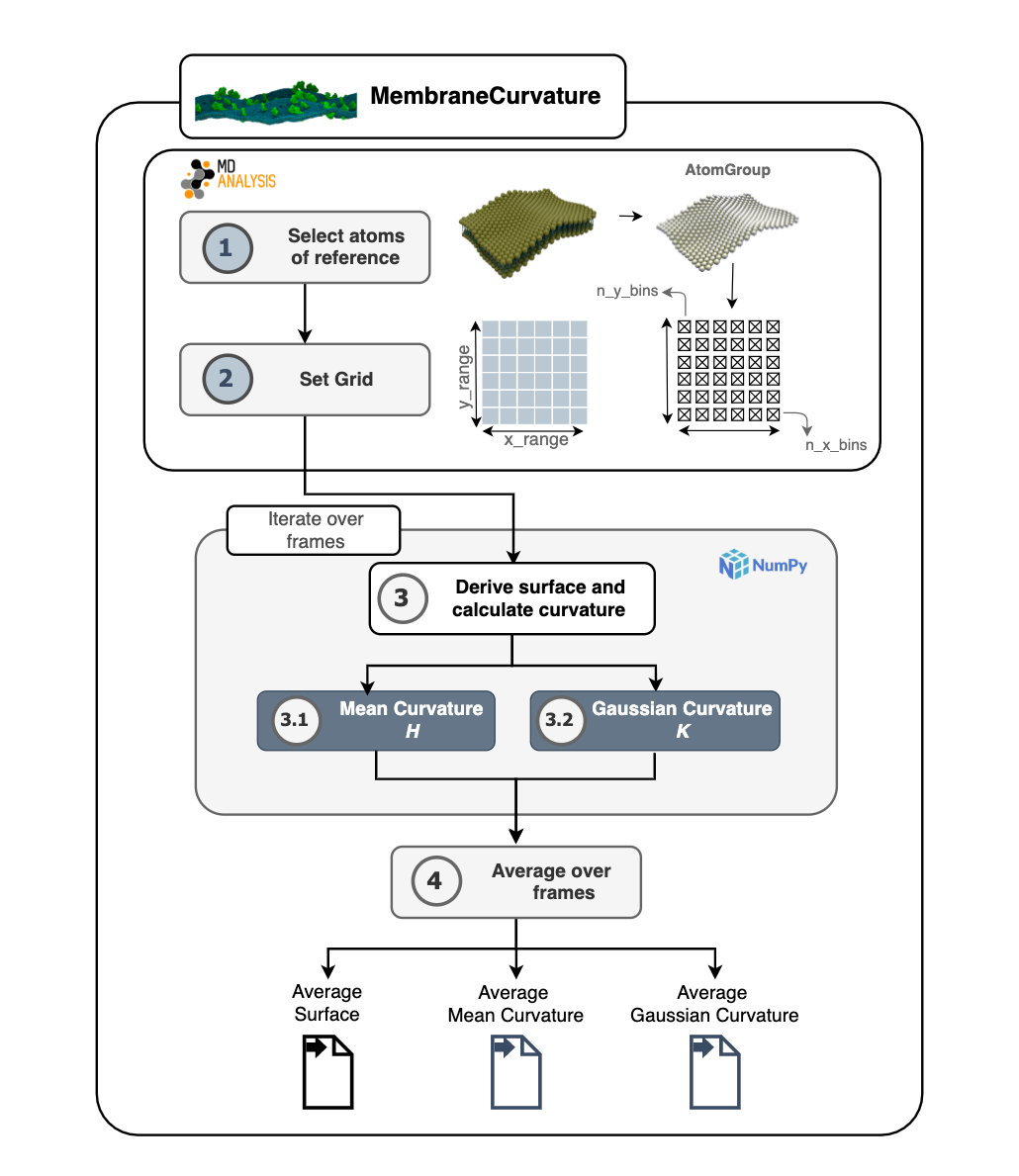
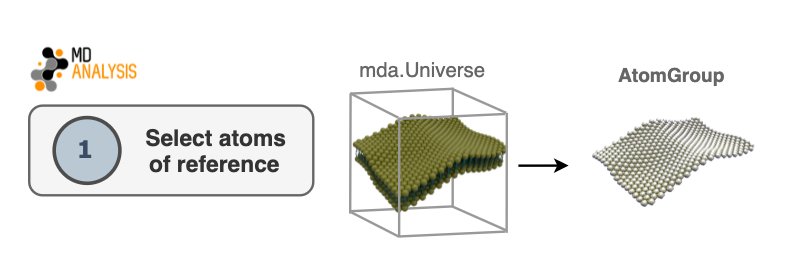
1. Select atoms of reference
The first step in the algorithm consists of selecting atoms that will be used as
a reference to derive a surface. This selection will be contained in an
AtomGroup. Typically in biological membranes,
lipid headgroups are the most common elements to use as an AtomGroup of
reference.
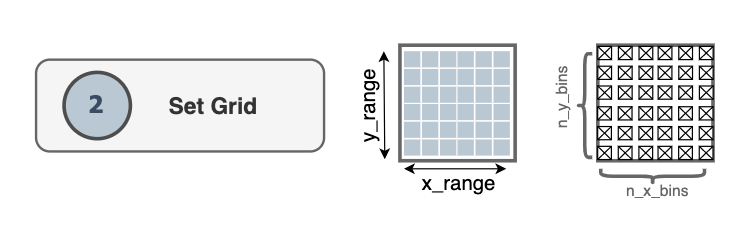
2. Set grid
The dimensions of the grid are determined by the size of the simulation box
contained in the Universe.
The grid covers a rectangular domain in the membrane plane. By default that
domain matches the x and y edges of the simulation box from MDAnalysis’
Universe.The grid comprises n_x_bins x
n_y_bins bins along the x and y directions.
For every atom in the AtomGroup of reference,
MembraneCurvature assigns it to a grid cell based on its x and y coordinates.
In practice, each coordinate pair (x, y) is mapped to a grid location
[l, m] corresponding to a bin in the discretized membrane surface.
Here, \(L_x\) and \(L_y\) represent the size of the region covered by
the grid along the x and y directions (i.e. the span of x_range and
y_range). The spacing between grid points in each direction is then
determined by dividing these lengths by the number of bins:
These spacings are used in derivative calculations so that curvature is computed in physical units.
Once the grid has been populated, the z coordinates of atoms assigned to each cell are collected to form a height field over the grid.
Note
Unless the user provides a different input, MembraneCurvature will determine
the dimensions of the grid based on the size of the box on the first frame via
dimensions.
grid_dimension_x = (0, universe.dimensions[0])
grid_dimension_y = (0, universe.dimensions[1])
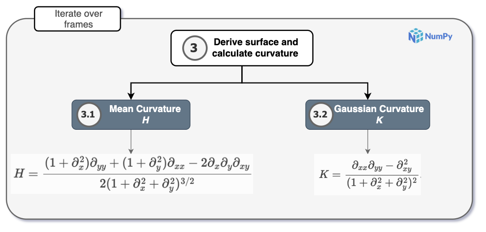
3. Derive surface and calculate surface derivatives
Once the surface formed by the atoms of reference is derived, mean (H) and
Gaussian (K) curvature are calculated from its spatial derivatives. These
derivatives are evaluated using the actual grid spacing (dx, dy), so that changes
in height are measured per unit distance in real space rather than per grid index.
This makes curvature values physically meaningful and reduces their sensitivity
to the chosen grid resolution.
Note
Curvature is computed from surface derivatives evaluated using the grid spacing
(dx, dy), ensuring results are expressed in physical units and are less
sensitive to grid resolution. Because the derivatives are computed numerically,
very coarse grids may still affect curvature estimates due to finite-difference
discretization error.
Curvature is obtained in two steps: partial derivatives of the height field on the
grid are estimated (for example with numpy.gradient() and box spacing), then
mapped to mean curvature \(H\) and Gaussian curvature \(K\) using the
Monge-gauge formulas in mean_curvature_monge()
and gaussian_curvature_monge().
For every frame of the trajectory, the surface derived from the
AtomGroup is
calculated and stored in z_surface.
Similarly, the calculation of mean and Gaussian curvature is performed in every
frame and stored in MembraneCurvature.results.mean_curvature and
MembraneCurvature.results.gaussian_curvature, respectively.
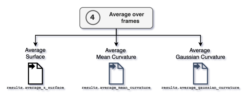
4. Average over frames
The attributes MembraneCurvature.results.average_mean and
MembraneCurvature.results.average_gaussian contain the computed
values of mean and Gaussian curvature averaged over all the
n_frames in the trajectory.
After performing the average over frames, the information of average surface,
mean, and Gaussian curvature are stored in the
MembraneCurvature.results.average_z_surface,
MembraneCurvature.results.average_mean, and
MembraneCurvature.results.average_gaussian arrays, respectively.
Each array has shape (n_x_bins, n_y_bins).